Brand Positioning using EFA and MDS

Supermarkets: the only differentiator is price
Exploratory Factor Analysis
In marketing, we are often interested in several key variables that cannot be measured directly, such as customer satisfaction with a product, purchase intent or category involvement. These factors are called latent variables, and they can be (somewhat imperfectly) assessed through their relationship to other variables, called manifest variables.
Manifest variables are, on the contrary, available indicators, such as responses to survey questions that ask about various aspects of customer experience, or empirical customer behavior, such as clicks in online shop.
The role of exploratory factor analysis or EFA is to establish a link between observed variables and latent variables, and to find out how much the composite variables account for the observed variance of the manifested variables.
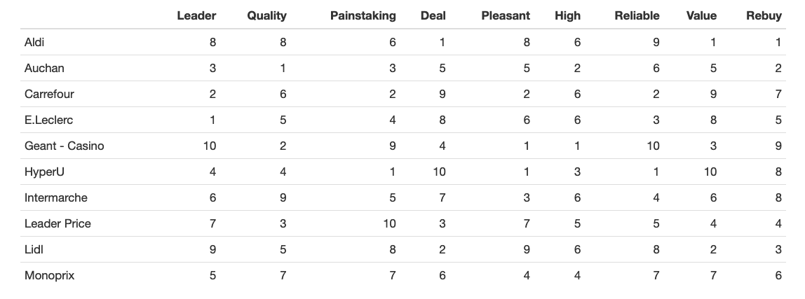
We will use the brand data from the previous article to uncover the latent dimensions in the data, and assess the brands in terms of those newly discovered factors.
EFA is rather different from PCA. While PCA focuses purely on transforming the dimensionality of the data, EFA focuses on its underlying latent dimensions. In other words, this principal difference is that EFA attempts to find solutions that are maximally interpretable in terms of the manifest variables. That makes it very valuable for business applications, because it allows the analyst to explain the results in ways that would be sometimes difficult with PCA, thus allowing decision-makers to act on the results.
For example, we might decide to keep the survey items that load on factor of interests and set aside the rest. We might also check whether the survey questions cover the reality successfully and whether the survey results correspond to expectations. We might learn, for instance, if the items of the given survey can and should be interpreted as a single factor (i.e. satisfaction), or if they in fact reflect multiple dimensions (i.e. quality satisfaction and service satisfaction that are quite different).
With this being said, EFA also serves as a data reduction technique for:
Simplifying data collection. By knowing the items that contribute highly to factor of interest, we can spare our data collection efforts by focusing on collecting data for important factors only.
Reducing noise. If we believe satisfaction is imperfectly reflected in several measures (and it usually is), the combination of those will have less noise than the set of individual items.
Dimensionality reduction. For example, we may use a single satisfaction score instead of several satisfaction scores.
Exploratory Factor Analysis of Supermarket Brands’ Perception
We will use the same dataset as in the previous article. You might want to check the data description and various considerations about it before reading further.
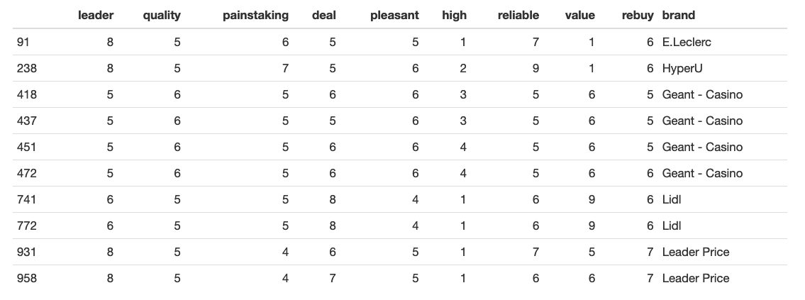
Just like with PCA, we will scale tha data first, and then we’ll see how many factors are present in the data, according to different methods:
| noc | naf | nparallel | nkaiser | |
|---|---|---|---|---|
| Suggested number of factors | 2 | 2 | 2 | 2 |
We can examine the eigen-values focusing on those that are greater than 1.0:
3.842, 2.763, 0.9493, 0.4774, 0.4304, 0.2177, 0.1568, 0.1167 and 0.04661
An eigen-value of 1.0 corresponds to the amount of variance that is attributed to a single independent variable, so anything below 1.0 is considered uninteresting. Based on that knowledge, we may believe again that there are two factors present. Let us examine this suggestion:
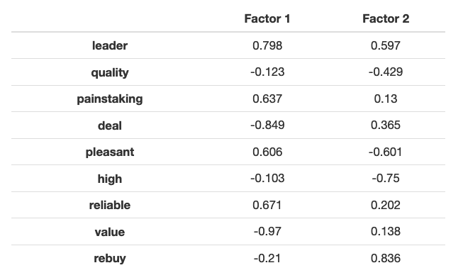
The Factor 1 makes good sense as focusing on perception of brand leader, but Factor 2 doesn’t look right to me. Keeping in mind that the third eigen-value was nearly 1.0, I try a 3-factor solution:
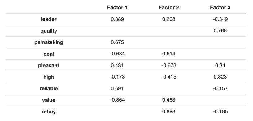
Factor 1 loads strongly on “leader” and “reliable” and therefore might be interpreted as a “leader” factor. Factor 2 is focused on “rebuy”, “value” and “deal”. Factor 3 loads on “high-end” and “quality” and thus might be regarded as a “quality” factor.
Notice that even though in the survey there was a significant positive correlation between manifested desire to rebuy and between all three of the “leader”, “rebuy” and “value” factors, our factor analysis shows that customers are mostly ready to rebuy for good value for money, and not for quality or reliability. This might be because the ‘quality’ keyword was mistranslated, while in fact it meant superiority in a different sense. Or, this might be because we’re trying to see the factors as independent, while in fact this might not be the case. We will address this issue in a moment.
Despite this consideration, the model adds a clearly interpretable concept to our understanding of the data and aligns well with examination of perceptual maps that we’ve seen in the previous article. It also shows that even though screeplot and eigen-values agree that there are TWO factors present, Marketing Data Scientist should always rely on business sense while interpreting the results and making suggestions for the managers.
Exporatory Factor Analysis with Dependent Factors
While doing EFA, the most critical question that the Data Scientist faces (after the interpretability of the results, of course), is the factor independance. Simply put, do I wish to allow the factors to be correlated or not? Do I think the factors should be conceptually independent, or does it make more sense to consider them to be related?
For instance, best value and market leader are most likely correlated. The leader is clearly in position to charge premium price, and so is likely to be strongly negatively correlated with best value. In some markets, it is quality, and not the market share that might be correlated to the perception of brand leader.
EFA with dependent factors is performed using oblique rotation:
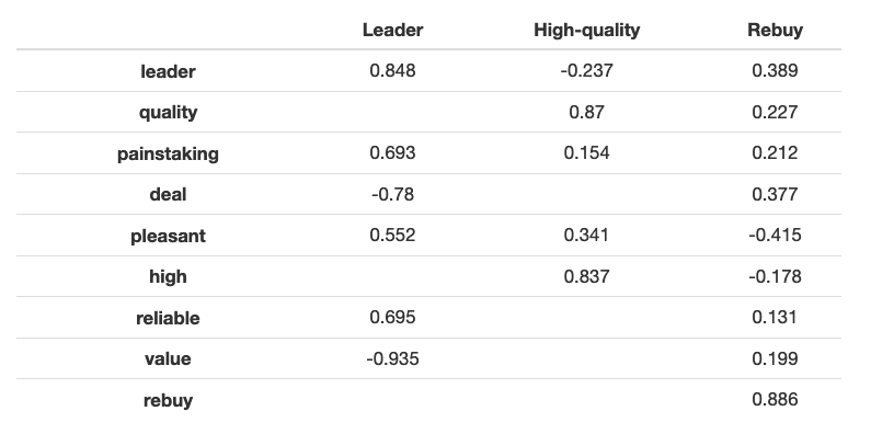
Notice this distinct separation into three factors, with consumer saying that they would rebuy for either reason, for good price or from a market leader.
Here again the results show three well defined factors: the “leader” factor, the “high-quality” factor and the “rebuy” factor (that we see here, is clearly correlated to both “deal” and “leader”, and in lesser degree, “quality”).
These findings seem to describe the reality better than the previous model that assumed that the factors were ortogonal (uncorrelated).
This example shows that understanding of the business problem is critical for the choice of the model. True Data Scientist’s job is much more about understanding the problem at hand and interpreting the results correctly, than about writing the code. If the scope of the business problem is beyond the analyst’s knowledge, questions must be adressed to the managers who order the analysis and who have this necessary vision.
Let us have a look at the graphical representation of the factor loadings.

The results can also be represented as the path diagram, which shows latent variables and the individual items (manifest variables) that contribute to them (or, better say, are related to them, as we might prefer to avoid the notion of causality).

The result of the EFA for this data set is that instead of using NINE manifest variables, we might instead represent the data with THREE underlying latent factors. This reduction of factors greatly reduces the complexity of the model. This can be useful if later on we wish to investigate the relationship of factors to demographics or purchase behaviour, or for regression or segmentation problems.
We can use the factor scores to determine brands’ positioning in regards to these factors. The result is an estimated score for each respondent on each factor and brand.
| Leader | Quality | Rebuy | |
|---|---|---|---|
| Aldi | -1.412 | -0.7049 | 1.452 |
| Auchan | 0.6569 | 1.245 | 1.032 |
| Carrefour | 0.8478 | -0.4525 | -0.3747 |
| E.Leclerc | 0.8324 | -0.5697 | 0.1143 |
| Geant - Casino | -1.121 | 2.373 | -2.081 |
| HyperU | 1.085 | 0.6011 | -0.4105 |
| Intermarche | 0.5504 | -1.091 | -0.6946 |
| Leader Price | -0.3958 | -0.4036 | 0.52 |
| Lidl | -1.687 | -0.5594 | 0.6976 |
| Monoprix | 0.6431 | -0.4382 | -0.2553 |
Represented graphically as a heatmap, it gives the following:

When we compare it to the intial heatmap, we can see that somehow it is much simpler and easier to examine, even though the structure stays similar.
To conclude, EFA is a great way to examine the underlying structure and relationship of factors. When items are related to some underlying constructs, EFA reduces data complexity by aggregating variables to create simpler, more interpretable latent variables.
Brand Positioning using Multi-dimensional Scaling
Principal Components Analysis is a robust and valuable method. It is also a more informative procedure than MDS for typical metric (or near-metric, such as Likert scale) data. However, when the data is non-metric, PCA won’t work and MDS is its valuable alternative.
So, to illustrate the multi-dimensional scaling applications, I will use the create non-metric MDS (like if we only had ranking data). To do so, I will convert the initial dataset into mean rankings aggregated by brand and by perception (see below):
I then run the MDS algorithm with gower metric, which is used for mixed numeric, ordinal, and nominal data. The isoMDS model output is below:
                                initial  value 11.788624
                                iter   5 value 7.777615
                                iter  10 value 7.535702
                                final  value 7.504845
                                converged
Finally, this is what graphical representation of the model output looks like:

If you try running metric MDS, as we could here, the resulting plot will be a bit different, because some of the data was lost when we converted to ranks. The general structure stays the same, however.
To summarize, MDS output is simple and gives less insights, but the method is very stable and works with non-metric data, where other algorithms won’t work. It may be of particular interest when the surveys aren’t available and we’re doing some data mining (for consumer’s feedback, comments, online reviews). For example, text frequencies can be converted to distance scores and used as MDS input. Coincidentally, text data mining might turn out to be more reliable data than surveys that are frequently biased, or suffer from imperfectly random sampling. One needs to account for the fact, however, that customers are more prone to writing negative reviews than positive ones.
Another way to look at similarities between brands is to count how many times two brands appear in the review together, then use this matrix of counts as the distance metric in MDS.
3 Comments
I still don't understand. How is this method better than the one in the article just before?
Do you mean EFA or MDS? MDS is better because it tells us something when other methods won't work at all (some information is better than none, I think). EFA isn't better, it's different. We were lucky that with this dataset PCA results can be interpreted with common sense. It is not always the case. Sometimes we end up with first two PCA dimensions that explain most of the factors, but have absolutely no business sense. EFA deals with this, because its dimensions are always some interpretable latent factors.